Marching Cubes and Metaballs (and an opengl implementation)
Whats our goal?
In this blog post im going to explore metaballs and how we can draw them using the marching squares algorithm. You have probably seen metaballs in one form or another whether it be in software, animations or games. It is a very cool visual effect that resembles many bubbles joining and splitting off from each other, which makes for awesome wallpapers or lava lamp visuals as well as many other applications in games and software.
Below is the final implementation of the metaballs using the method in this blog post, this is where we are headed.
Defining a metaball
Now in order to implement these we must define what the metaball actually is. The metaball is a point on a 2D grid, it has a certain strength value (you can think of it as a radius of some sort) and its x and y coordinates.
We can start with the equation of a circle
\[(x - x_0)^2 + (y - y_0)^2 = r^2\]Where \((x_0, y_0)\) is the center of the circle and r is the radius. We can rearrange the values to get the equation in another form
\[1 = \frac{r^2}{(x - x_0)^2 + (y - y_0)^2}\]This equation tells us that when the the value of the function is greater than one, it lies inside the circle, and when it is less than one it lies outside as it is only 1 exactly inside the circle.
However, to get the signature bubble feel from the metaball we take the sum of all these functions for each point
\[f(x, y) = \sum_{i=1}^{n} \frac{r_i^2}{(x - x_i)^2 + (y - y_i)^2}\]Where n is the number of metaballs in the scene.
Here is how we could implement this in code (taking the sum of all the inverse distances to each metaball):
calculateValueAtPoint(x, y):
    sum = 0
    for each metaball in metaballs:
        dx = x - metaball.x
        dy = y - metaball.y
        sum += metaball.strength / (dx*dx + dy*dy)
    return sum
This gives us the value of each metaball at a point if we iterate over all x and y coordinates, now we just have to visualize this in our code.
We can visualize this on desmos, check out the interactive example below.
You can move the points around by clicking and dragging
As you move around the sliders for the x1, x2, y1, and y2 positions you will see that the line drawn when the the points are equal to 1 changes smoothly.
Drawing metaballs
So how do we actually render these metaballs in a program? We have a function that we want to plot points if the value is equal to 1.
First Approach: Checking each pixel
The first approach that comes to mind would be to iterate over every pixel and use the calculateValueAtPoint(x,y) function to determine if the pixel is equal 1 or not. If it is equal 1 then we can color that pixel in. This doesn’t work in practice however because the value usually never sums up to 1 exactly, so we define a threshold around 1 to check if the pixel is colored in.
Heres some psuedo code as to how you would implement this
for each pixel in the screen:
    value = calculateValueAtPoint(pixel.x, pixel.y)
    if value > 0.9 and value < 1.1:
        colorPixel(pixel)
Here is the actual implementation in C++ which is given the start pixel index and the end pixel index (if your pixel is the last one then it would be width * height).
// Calculating the value of each pixel using a 2D array
void calculatePowerThread(int start, int end){
    for (int i = start; i <= end; i++){
        int x = convertArrX(i);
        int y = convertArrY(i);

        float xPos = x - 0.5;
        float yPos = y - 0.5;
        for(int i = 0; i < metaBalls.size(); i++){
            sums[x][y] += metaBalls[i].scale/(length(metaBalls[i].x, metaBalls[i].y, x, y));
        }
    }
}

void drawAllPixels(){
    // Drawing the pixels (found inside the main draw loop)
    for(int i = 0; i < screenWidth; i++){
        for(int j = 0; j < screenHeight; j++){
            if (sums[i][j] > 0.99 && sums[i][j] < 1.01){
                DrawRectangle(i, j, 1, 1, BLUE); // Assuming each cell is a pixel so it has a width and height of one
            }
        }
    }
}
You can find the full source here (uses C++ and raylib)
This approach has some issues:
- We have to define threshold around the value of 1 which doesn’t maintain its accuracy if we zoom
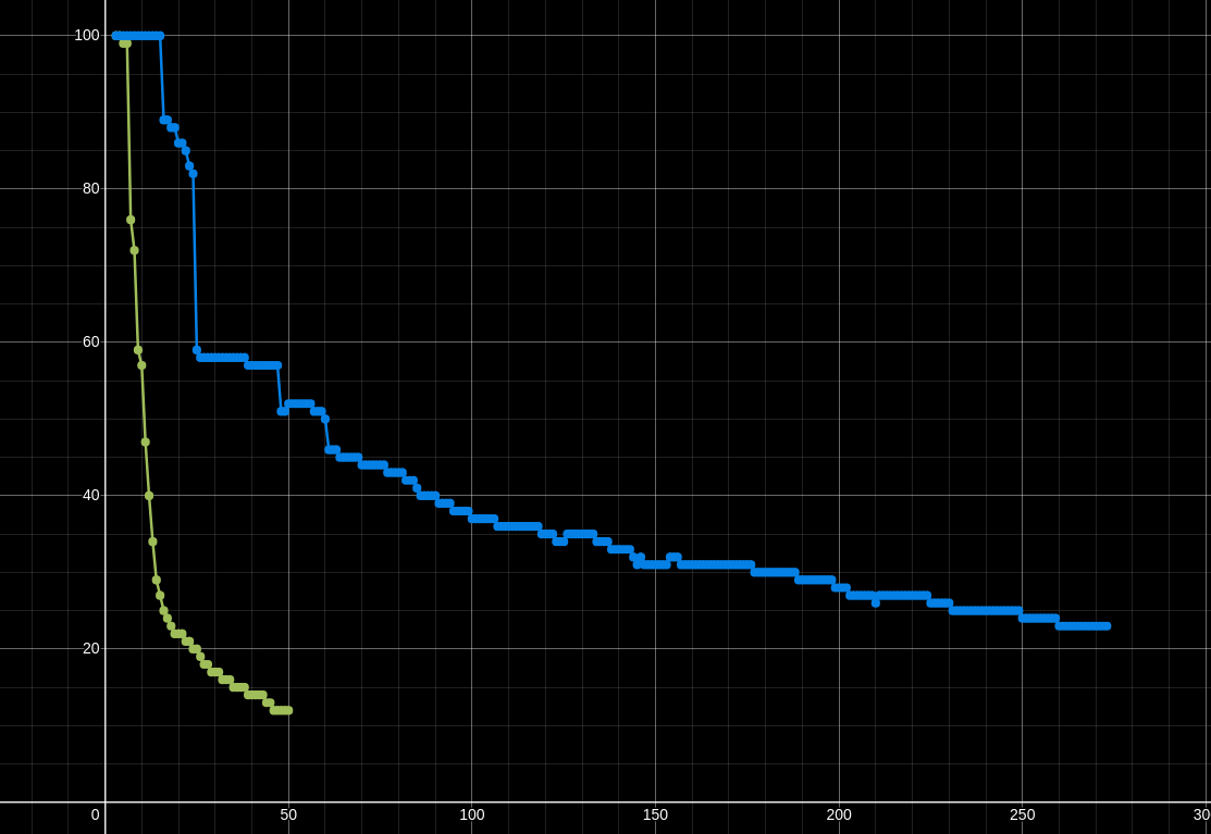
- Poor performance: the FPS drops significantly as we increase the number of metaballs, here is some data on the performance
To try and fix this we could try multithreading and splitting the work between the CPU cores. This does have a performance benefit increase but it still can’t handle as many metaballs as I would like.
Heres an example solution using the same code from above:
// Used for keeping track of each sum
float sums[screenWidth][screenHeight];

void calculatePixelsThread(int start, int end){
    for (int i = start; i <= end; i++){
        int x = convertArrX(i);
        int y = convertArrY(i);

        float xPos = x - 0.5;
        float yPos = y - 0.5;
        for(int i = 0; i < metaBalls.size(); i++){
            sums[x][y] += metaBalls[i].scale/(length(metaBalls[i].x, metaBalls[i].y, x, y));
        }
    }
}

void calculateEachPixel(){
    for(int i = 0; i < screenWidth; i++){
        for(int j = 0; j < screenHeight; j++){
            sums[i][j] = 0;
        }
    }

    // convert x and y into actual coords
    int numThreads = 8;
    int totalSize = screenHeight * screenWidth;
    int countPerThread = totalSize / numThreads;

    vector<thread> calculationThreads;
    for (int i = 0; i < numThreads; i++){
        // Start a new thread with the correct index range for the pixels
        calculationThreads.push_back(thread(calculatePixelsThread, i*countPerThread, (i+1)*countPerThread));
    }

    for (int i = 0; i < numThreads; i++){
        calculationThreads[i].join(); // Wait for each thread to terminate
    }
}
Heres how the performance looks when compared to the amount of metaballs (blue is multithreaded, and green is single threaded). The x axis is the amount of metaballs and y axis the frame rate.
Second Approach: Marching Squares
The second approach puts a clever twist on the original implementation. Instead of just coloring the whole cell based on its center value (x,y), we can instead use several test values to see which corners of the cell are inside or outside of the cell. What this allows for is a much larger cell size and a more accurate representation of the metaballs, while also eliminating the need for a threshold.
For one cell (see below) we calculate each of the corners, then we can determine which corners are inside the metaball or not (greater than 1 is inside, less than 1 is outside of the metaball). Which gives us enough information to draw a line of where the metaball is.
This leaves us with 16 cases that we need to cover in order to draw the metaball in its entirety.
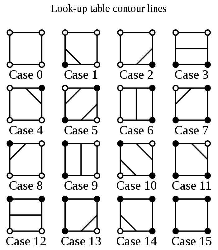
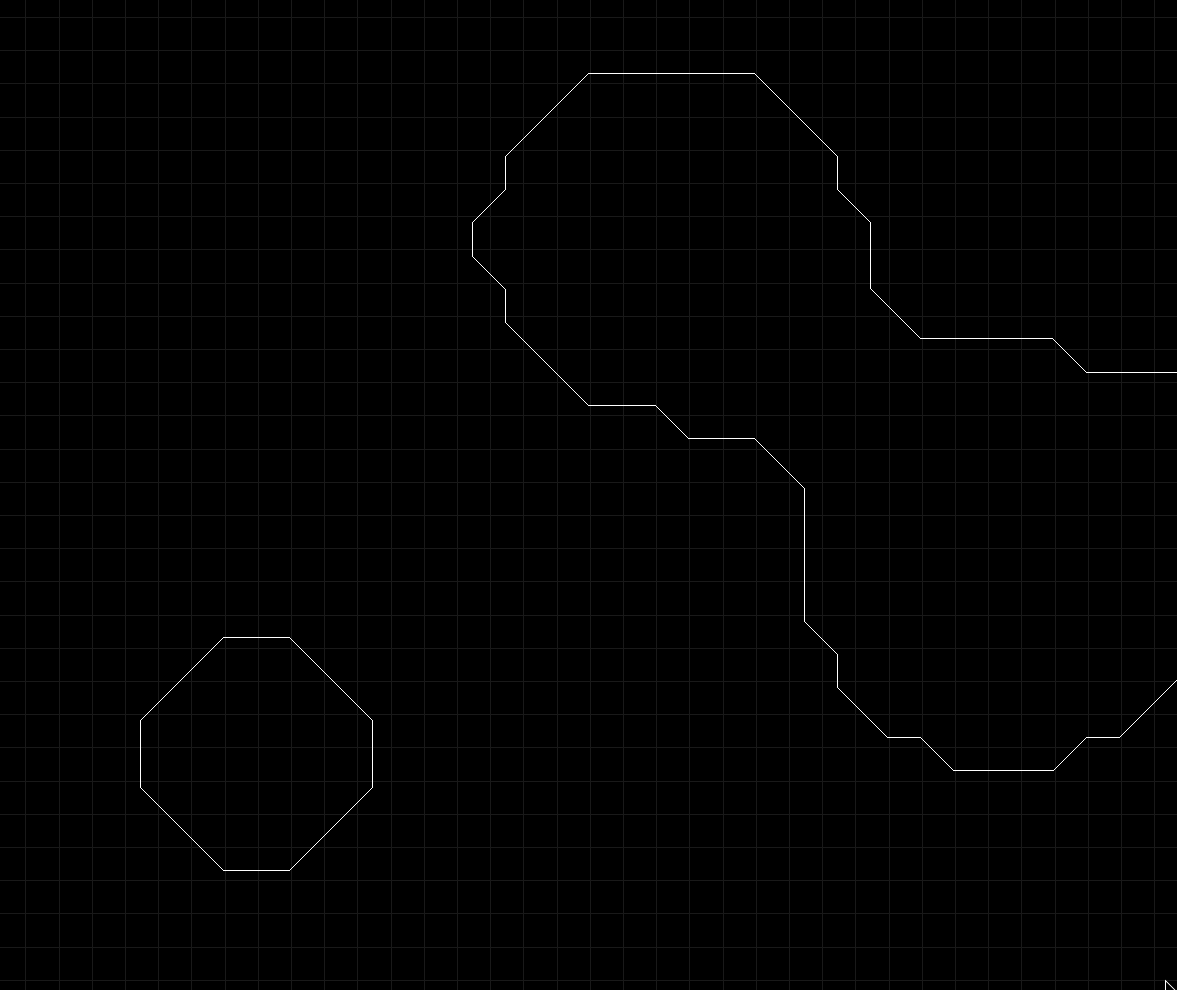
With these cases we loop over each cell to determine which of the 16 cases it is and draw the according lines to the screen. This results in a blocky looking approximation of our metaballs, but it performs a lot faster.
Here is the visualization of this approach:
How can we improve this?
This clearly has some issues, it looks too blocky! What we do know is for each cell that has a corner inside the metaball, there exists a solution to our equation such that the x (or y position) is equal exactly to one. However, finding the root for this equation is very slow so instead we make a linear approximation.
How do we do this exactly? Lets take a look at the example below
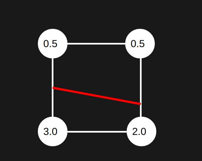
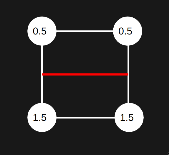
We first assume it will be a linear relation between the two points which is a good enough approximation for our use case (lets look at the top right and bottom right corners).
We will set some input t, which will be the percent along the line between the two points. This lets us write out an equation for the linear interpolation.
\[\text{Interpolation}(t) = p1 + (p2 - p1) * t\] \[\text{Interpolation}(t) = 0.5 + (2.0 - 0.5) * t\]So when \(t=1\) then we get the bottom right corner as our output, and when \(t=0\) we get the top right corner value. We want to solve for when the output is equal to one, so we set \(\text{Interpolation}(t) = 1\) and solve for t.
\[1 = p_{outer} + (p_{inner} - p_{outer}) * t\] \[1 - p_{outer} = (p_{inner} - p_{outer}) * t\] \[t = \frac{1 - p_{outer}}{p_{inner} - p_{outer}}\]Now that we’ve solved for t, we can find what y (or x) value is needed to make the value equal to 1 using our linear approximation. So we take T and multiply it by the size of the cell to get the actual offset from the corner that we were analyzing. In this case we step up the y value by \(t \cdot cellSize\) to get the actual y value that we need to draw the line at.
Lets apply this formula to our example above.
\[t = \frac{1 - 0.5}{2.0 - 0.5} = \frac{1}{3}\] \[Y_{solved} = Y_{original} + \text{sizeOfCell} \cdot \frac{1}{3}\]We are adding in this case because the point inside the metaball lies below the point outside the metaball
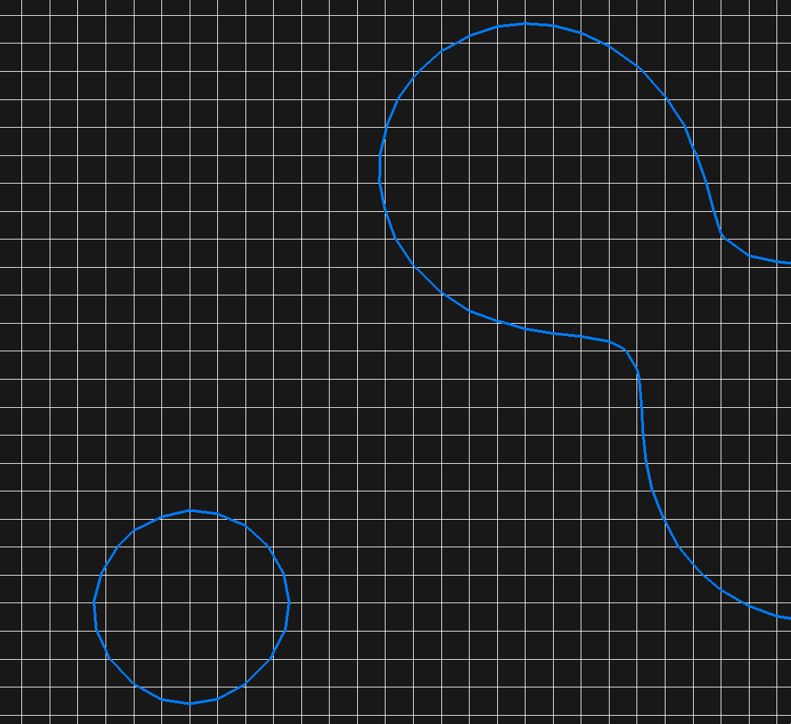
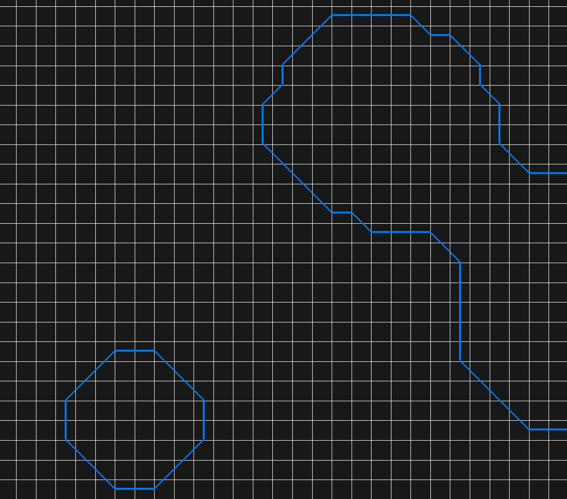
Applying this to our marching squares algorithm gives a much cleaner approximation of the metaballs as the linear approximation is close enough to the actual value.
Heres a side by side comparison with the linear interpolation and without.
Performance of marching cubes (with compute shader)
The performance of the marching cubes algorithm is a lot better when paired with a compute shader (a program that allows to compute many things in parallel independently of each other). The compute shader calculates the value of each corner of each cell and then it runs a vertex shader that determines which case it is in.
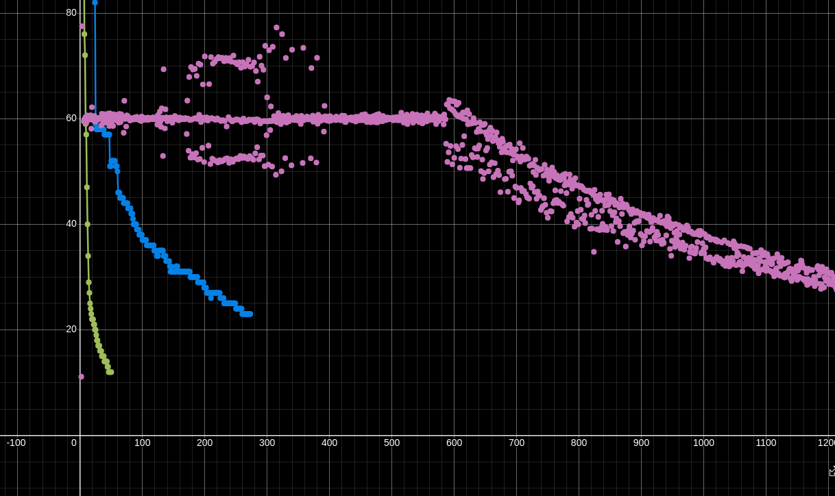
Here is a comparison of the performance of the marching cubes algorithm with and without the compute shader
You can find the full source here (uses opengl and C++)
Blue is multithreaded, green is single threaded, purple is using a compute shader, x axis is # of metaballs, y axis is frames per second